Announcing the Launch of the AI/ML Enhancement Project for GEP and Urban TEP Exploitation Platforms

[simonevaccari]

AI/ML Enhancement Project - Labelling EO Data User Scenario 2

Introduction

Labelling data is a crucial step in the process for developing supervised Machine Learning (ML) models. It involves the critical task of assigning relevant labels or categories to different features within the data, such as land cover class (e.g. vegetation, water bodies, urban area, etc.) or other physical characteristics of the Earth’s surface. These labels can be multi-class (e.g., forest, grassland, urban), or binary (e.g., water or non-water).

This post presents User Scenario 2 of the AI/ML Enhancement Project, titled “Alice labels Earth Observation (EO) data”. It demonstrates how the enhancements being deployed in the Geohazards Exploitation Platform (GEP) and Urban Thematic Exploitation Platform (U-TEP) will support users labelling EO data.

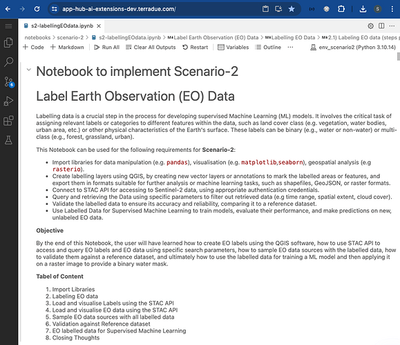
For this User Scenario, an interactive Jupyter Notebook is used to guide an ML practitioner, such as Alice, through the following steps:

• create data labels, using QGIS Software or a Solara / Leafmap application
• load Labels and Sentinel-2 data using STAC API
• sample Sentinel-2 data with Labels and create a dataframe
• validate the labelled data against the Global Surface Water (GSW) dataset
• use the dataframe to train a ML model based on a Random Forest classifier
• perform raster inference on a Sentinel-2 scene to generate a binary water mask

Practical examples and commands are displayed to demonstrate how this new capabilities can be used from a Jupyter Notebook.

Labelling EO data

The process for creating vector (point or polygon) data layers is illustrated with two examples:

• QGIS Software: a dedicated profile on the App Hub is configured to the user for using QGIS Software (more details can be found on the App Hub online User Manual). The steps to create new Shapefile Layers, add classification types for each point / polygon, and save the output in a geojson format are illustrated with several screenshots.
• Solara / Leafmap application: an interactive map, built on Solara and Leafmap, has been integrated in the Notebook to give the option to the user to manually create and save labels right from the Notebook itself.

After the annotations are created, either from QGIS or from the Solara / Leafmap interactive map, and saved into a .geojson file, the user can create the STAC Item of the EO labels, and publish it on the STAC endpoint. This is done with the pystac Python library and an interactive form right in the Notebook.

Load Labels and EO data with STAC API

Access to Labels and EO data was facilitated through the utilisation of the libraries pystac and pystac_client. These libraries enable users to interact with a STAC catalog by defining specific query parameters, such as time range, area of interest, and data collection preferences. Subsequently, only the STAC Items that align with the provided criteria are retrieved for the user.

Below is given a simplified code snippet for implementing STAC data search and for displaying results on an interactive map. An upcoming article, dedicated to the STAC format and data access will be published, with more guidance and examples.

Search data using STAC API

# Import libraries
import pystac; from pystac_client import Client

# Access to STAC Catalog
cat = Client.open("https://ai-extensions-stac.terradue.com", ...)

# Define query parameters
start_date = “2023-06-01”
end_date = “2023-06-30”
bbox = [-121.857043 37.853934 -120.608968 38.840424]
cloud_cover = 30
tile = “10SFH”

# Search Labels by AOI, start/end date
query_sel = cat.search(
  collections=[“ai-extensions-svv-dataset-labels”],
  datetime=(start_date, end_date),
  bbox=bbox,
)

labels = query_sel.item_collection()

# Search EO data (Sentinel-2) by AOI, start/end date, cloud cover and tile number
query_sel = cat.search(
  collections=[“sentinel-2-l2a”],
  datetime=(start_date, end_date),
  bbox=bbox,
  query={"eo:cloud_cover": {"lt": cloud_cover}},
)

eo_item = [item for item in query_sel.item_collection() if tile in item.id][0]

Plot Labels and EO data on interactive map

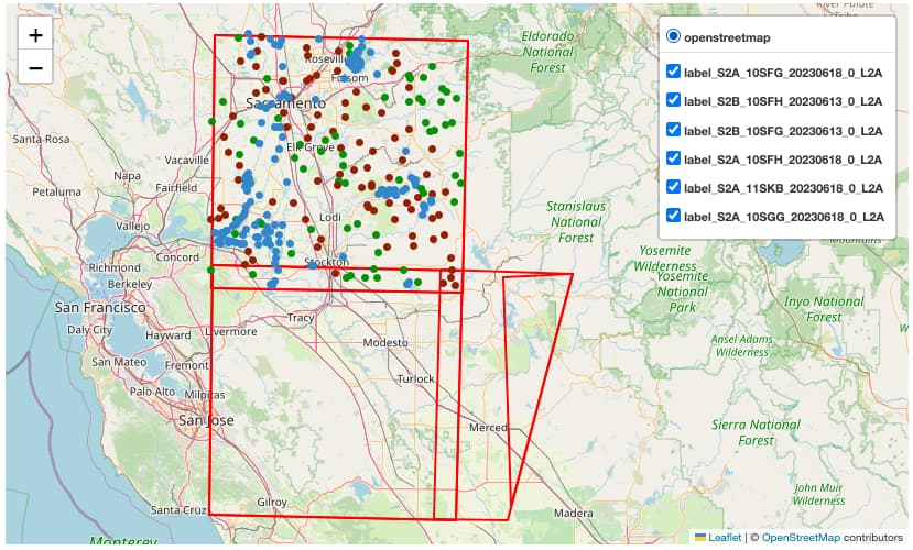
Once the Label data is loaded, it is converted into a dataframe (gdf) using geopandas library. The Python library folium was then used to display both the Labels and EO data on an interactive map.

import folium; from folium import GeoJson, LayerControl, plugins

map = folium.Map(location=[x, y], tiles="OpenStreetMap", zoom_start=9)

# Add Labels to map
map = addPoints2Map(gdf, map)

# Add footprint of EO scene
footprint_eo = folium.GeoJson(eo_item.geometry,style_function=lambda x: {...})
footprint_eo.add_to(map)

# Visualise map
map

Sample EO data with labels

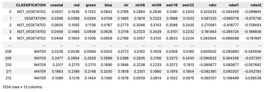
After loading the data, the Notebook continues with the implementation of a function to iteratively sample the EO data in correspondence of each labelled point. In addition to sampling a selection of the Sentinel-2 reflectance band (coastal, red, green, blue, nir, nir08, nir09, swir16, and swir22), three vegetation indices are also calculated (ndvi, ndwi1, and ndwi2). After sampling the EO bands and calculating the vegetation indices, all the data is concatenated into a pandas DataFrame.

import pandas as pd

tmp_gdfs = []
for i, label_item in enumerate(eo_items):
  sampled_data = sample_data(label_item=label_item, common_bands=["coastal", "red", "green", "blue", "nir", "nir08", "nir09", "swir16", "swir22"])
  tmp_gdfs.append(sampled_data)

# Create pandas dataframe
gdf_points = pd.concat(tmp_gdfs)

# Save to file
gdf_points.to_pickle(“filename.pkl”)

Validation against Reference Dataset

A comparison against another, independent, dataset was performed to show a validation approach of the labelled data. As a validation dataset, we used the Global Surface Water (GSW) dataset, generated by JRC (Citation: Pekel, Jean-François; Cottam, Andrew; Gorelick, Noel; Belward, Alan (2017): Global Surface Water Explorer dataset. European Commission, Joint Research Centre (JRC), http://data.europa.eu/89h/jrc-gswe-global-surface-water-explorer-v1).

The comparison was performed simply by iterating through the generated labels dataframe and by counting the number of points labelled as “water” that were correctly classified as water (i.e. with pixel value higher than 80%) also in the GSW dataset.

EO labelled data for Supervised ML task

Dataset preparation

The dataframe was prepared for the supervised ML task by converting it into a binary classification dataset (i.e. “water” and “no-water”) and by removing unnecessary columns. Further and more detailed analysis on the dataframe can be performed through Exploratory Data Analysis (EDA). Check out more information on the recently published article dedicated to EDA, for more details and guidance on this.

The dataset was then split into train and test with the dedicated function train_test_split() from the sklearn package.

from sklearn.model_selection import train_test_split

# columns used as features during training
feature_cols = ['coastal','red','green','blue','nir','nir08','nir09','swir16','swir22', 'ndvi', 'ndwi1', 'ndwi2']

# column name for label
LABEL_NAME = 'CLASSIFICATION'

features = train_dataset[feature_cols] # cols for features
label = train_dataset[LABEL_NAME] # col for labels
X_train, X_test, y_train, y_test = train_test_split(
  features, label,
  random_state=42,
  train_size=0.85,
)

ML Model

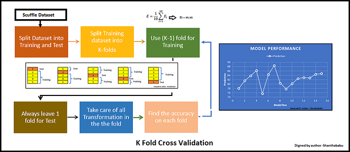
The ML model developed in this Notebook was a Random Forest classifier using k-fold cross validation. Random Forest is a powerful and versatile supervised ML algorithm that grows and combines multiple decision trees to create a “forest.” It can be used for both classification and regression problems. K-Fold Cross-Validation is a technique used in ML to assess the performance and generalisation ability of a model. The steps involved in the K-Fold Cross-Validation are:

1. split the dataset into K subsets, or “folds”.
2. The model is then trained K times, each time using K-1 folds for training, and the remaining fold for validation.
3. This process is repeated K times, with each of the K folds used exactly once as the validation data.
4. The K results from the K folds are then averaged to produce a single estimation of model performance.

The ML parameters are defined and used to train the model with a few simple functions, provided these are defined.

hyperparameters = {
  'n_estimators': 200,
  'criterion':'gini',
  'max_depth':None,
  'min_samples_split':2,
  'min_samples_leaf':1,
  'min_weight_fraction_leaf':0.0,
  'max_features':'sqrt',
  'max_leaf_nodes':None,
  'min_impurity_decrease':0.0,
  'bootstrap':True,
  'oob_score':False,
  'n_jobs':-1,
  'random_state':42,
  'verbose':0,
  'warm_start':True,
  'class_weight':None,
  'ccp_alpha':0.0,
  'max_samples':None
}

# define model obj which is defined in utils.py
model = Model(hyperparameters)

# training model using k-fold cross validation
estimators = model.training(X=X_train,Y=y_train,folds=5)

Model Evaluation

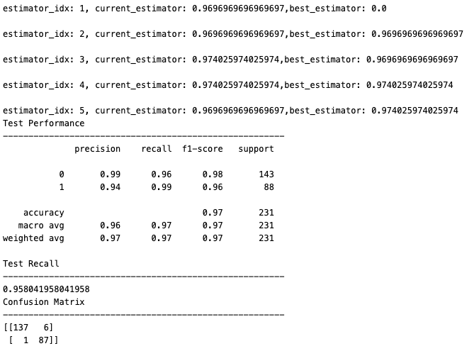
The model is evaluated on unseen data with the following evaluation metrics:

• Accuracy: calculated as the ratio of correctly predicted instances to the total number of instances in the dataset
• Recall: also known as sensitivity or true positive rate, recall is a metric that evaluates the ability of a classification model to correctly identify all relevant instances from a dataset
• Precision: it evaluates the accuracy of the positive predictions made by a classification model
• F1-score: it is a metric that combines precision and recall into a single value. It is particularly useful when there is an uneven class distribution (imbalanced classes) and provides a balance between precision and recall
• Confusion Matrix: it provides a detailed breakdown of the model’s performance, highlighting instances of correct and incorrect predictions.

The code snippet below shows how the model can be evaluated, followed by the output of the evaluation metrics calculated during the process.

# evaluate model
best_model = model.evaluation(estimators,X_test, y_test)

Other ways to evaluate the ML model are the distribution of the probability of predicted values, the Receiver Operating Characteristic (ROC) Curve, and the analysis of the permutation features importance. All three can be derived and plotted from within the Notebook with one simple line of code.

# Distribution of probability of predicted values
ml_helper.distribution_of_predicted_val(best_model, X_train, X_test)

# ROC Curve
ml_helper.roc(best_model,X_test,y_test)

# Permutation Importance
ml_helper.p_importance(best_model,X_test,y_test,hyperparameters,MODEL_OUTPUT_DIR)

Finally, the best ML model can be saved to a file so that it can be loaded and used in the future. The only prerequisite for applying the ML model is for the input dataset to have the same format as the training dataset described above.

import joblib

# Save the model to file
model_fname = 'best_rf_model.joblib'
joblib.dump(best_model, model_fname)

Raster Inference

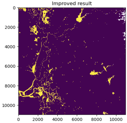
Now the user can apply the ML model on a Sentinel-2 image to generate a binary water mask output. After loading the EO data and the ML model into the Notebook, the ML model is applied to make predictions over the entire input EO data. The steps to perform these operations are shown in the simplified code snippet below.

# Select EO assets from the loaded Sentinel-2 scene (eo_item)

fileList = {}
for f in eo_item.get_assets():
  if (f in feature_cols) or f == 'scl':
    fileList[f] = eo_item.get_assets()[f].href

# Load the ML model classifier
model = joblib.load(model_fname)

# Make predictions
predictions = ml_helper.readRastersToArray(model, fileList, feature_cols)

# Save predictions
df_predict = pd.DataFrame(predictions.ravel(),columns=['predictions'])
df_predict.to_pickle('prediction.pkl')

# Create binary mask
predictions = df_predict['predictions']
predictions = predictions.to_numpy().reshape((10980,10980))

# Apply sieve operation to remove small features (in pixels)
my_array_uint8 = predictions.astype(rasterio.uint8)
sieved = sieve(my_array_uint8, threshold=1000, connectivity=8)

# Use Scene Classification band to filter out clouds and bad data
with rasterio.open(fileList['scl']) as scl_src:
  scl = scl_src.read(1)
  scl = np.where(~np.isin(scl, [4, 5, 6, 7, 11]), np.nan, scl)
mask_out = np.where(~np.isnan(scl), sieved, np.nan)

# Use Scene Classification band to filter out clouds and bad data
import matplotlib.pyplot as plt
plt.imshow(mask_out,interpolation='none'); plt.title("Improved result")

In the figure above, water bodies are plotted in yellow and non-water pixels are plotted in dark blue, and clouds are masked out in white (top-right corner of the image).

Conclusion

This work demonstrates the new functionalities brought by the AI/ML Enhancement Project to help a ML practitioner:

• create EO data labels, using QGIS Software or a Solara / Leafmap application
• load Labels and EO data with STAC API
• sample EO data with Labels and create a dataframe
• use the dataframe to train a Random Forest classifier
• perform raster inference on a selected Sentinel-2 scene to generate a binary water mask.

Useful links:

• The link to the Notebook for User Scenario 2 is: https://github.com/ai-extensions/notebooks/blob/main/scenario-2/s2-labellingEOdata.ipynb.
  Note: access to the Notebook for User Scenario 2 must be granted - please send an email to support@terradue.com with subject “Request Access to s2-labellingEOdata” and body “Please provide access to Notebook for AI Extensions User Scenario 2”
• The user manual of the AI/ML Enhancement Project Platform is available at AI-Extensions Application Hub - User Manual
• Link to the project update article “AI/ML Enhancement Project - Progress Update”
• Link to User Scenario 1 article “AI/ML Enhancement Project - Exploratory Data Analysis”