AI/ML Enhancement Project - Describing a trained ML model with STAC
Introduction
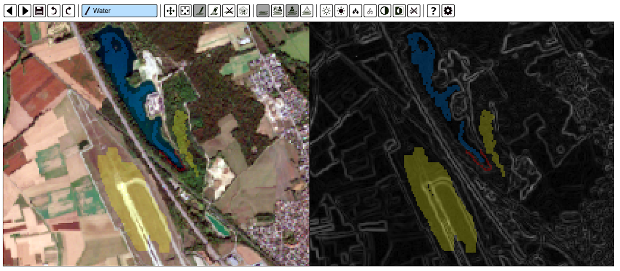
In this scenario, the ML practitioner Alice describes a trained ML model by leveraging the capabilities of the STAC format. By utilising STAC, Alice can describe her ML model by creating STAC Objects that encapsulates relevant metadata such as model name and version, model architecture and training process, specifications of inputs and output data formats, and hyperparameters. The STAC Objects can then be shared and published so that it can be discovered and accessed effectively. This enables Alice to provide a comprehensive and standardised description of her model, facilitating collaboration but also promoting interoperability within the geospatial and ML communities.
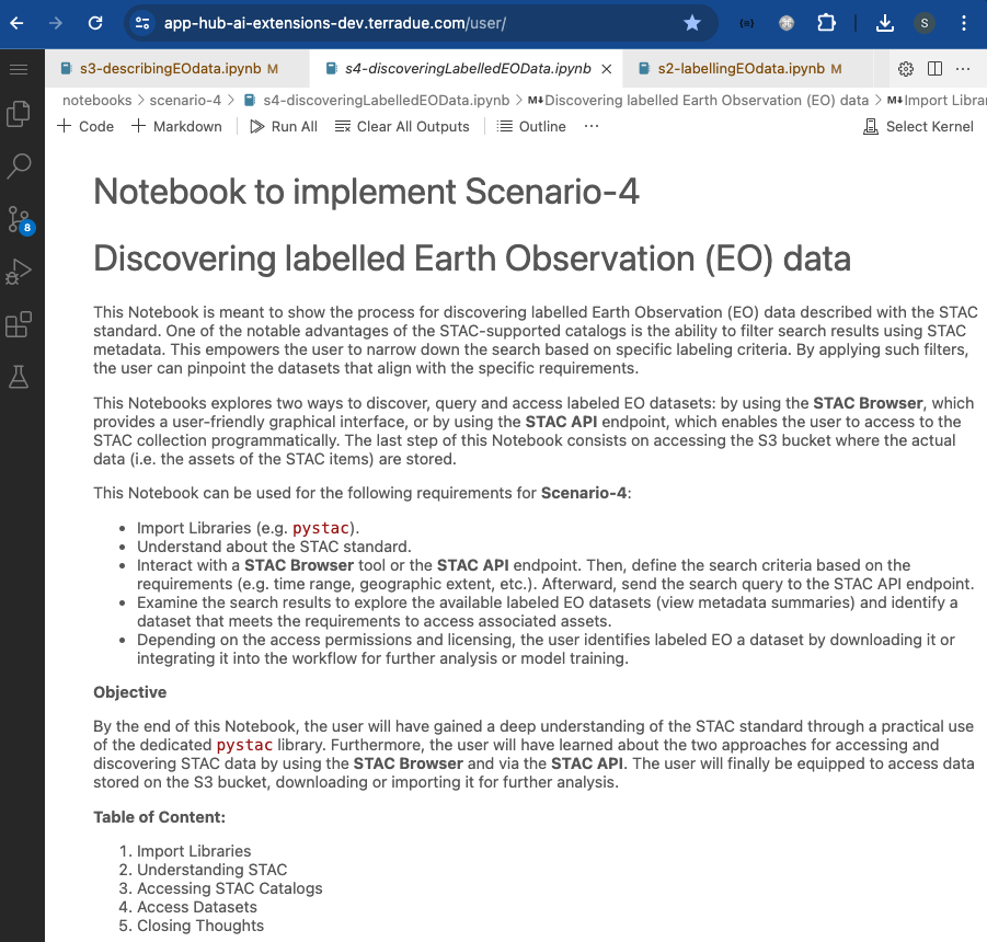
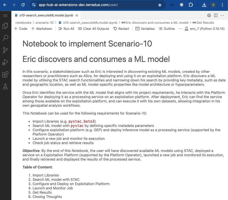
This post presents User Scenario 7 of the AI/ML Enhancement Project, titled “Alice describes her trained ML model”. It demonstrates how the enhancements being deployed in the Geohazards Exploitation Platform (GEP) and Urban Thematic Exploitation Platform (U-TEP) will support users on describing an ML model using the STAC format and the ML-dedicated STAC Extensions.
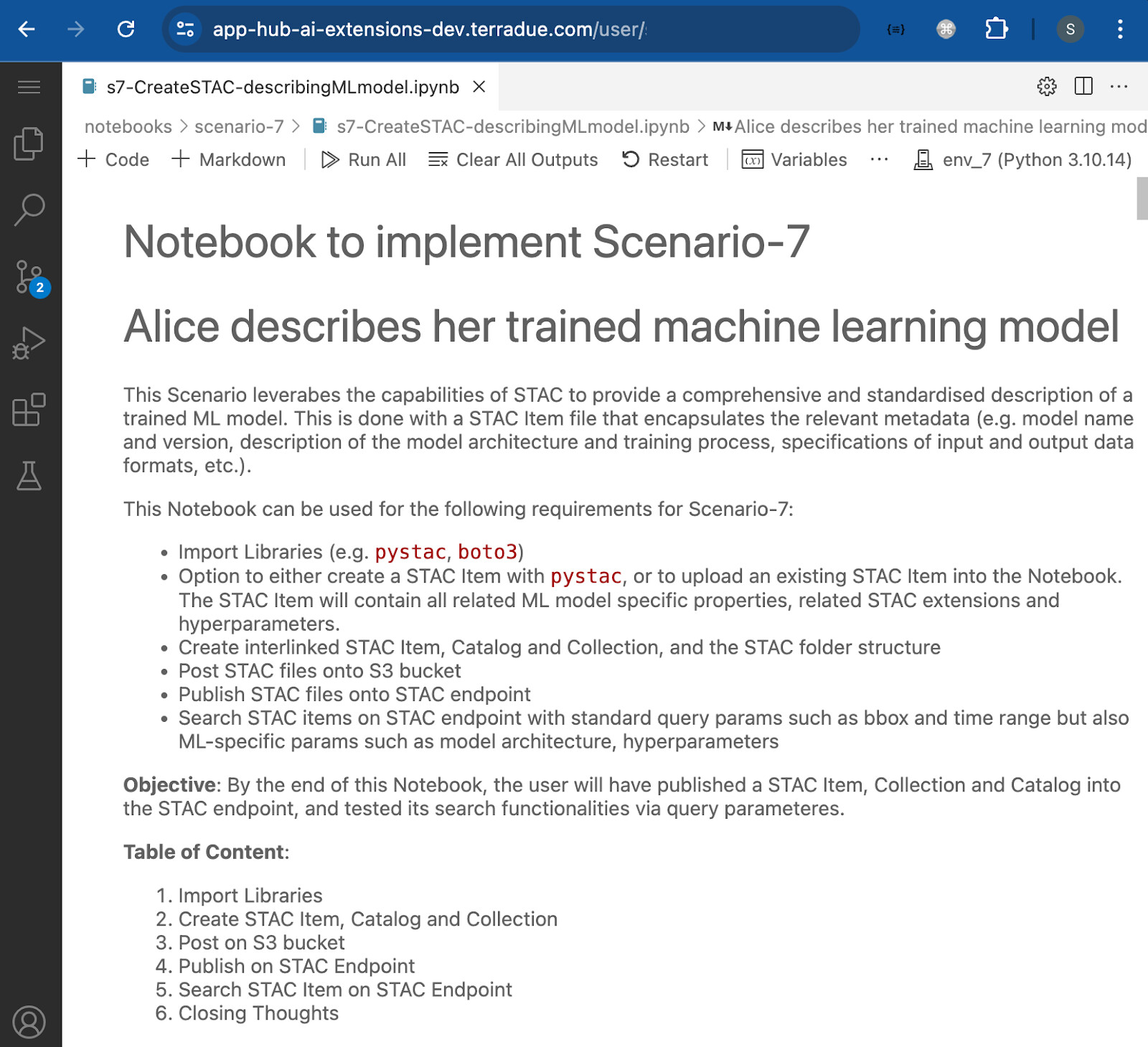
These new capabilities are implemented with an interactive Jupyter Notebook to guide an ML practitioner, such as Alice, through the following steps:
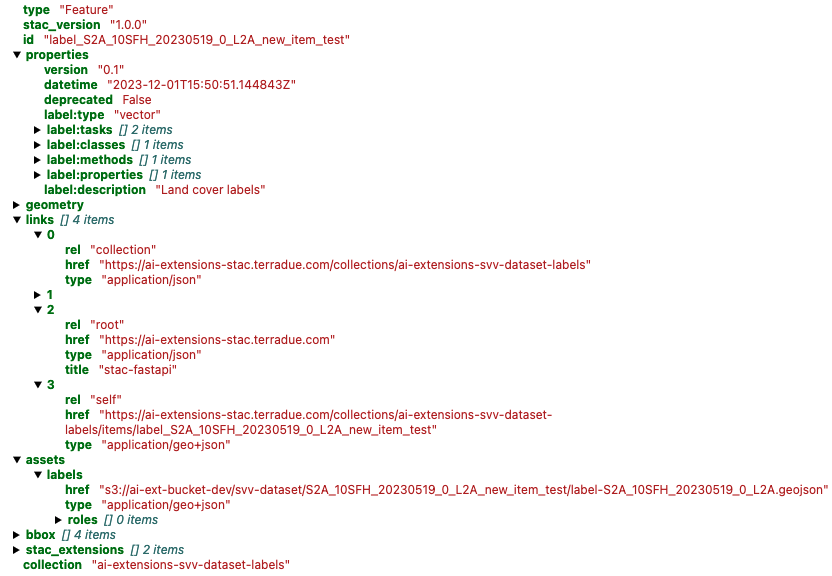
- Create a STAC Item, either with
pystac or by uploading an existing STAC Item into the Notebook, and its related Catalog and Collection. The STAC Item contains all related ML model specific properties, related STAC extensions and hyperparameters.
- Post STAC Objects onto S3 bucket
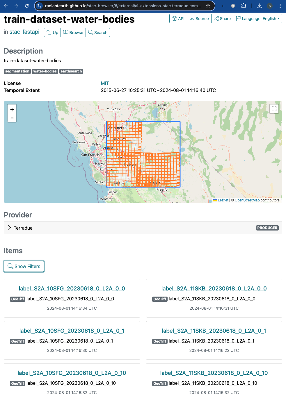
- Publish STAC Objects onto STAC endpoint
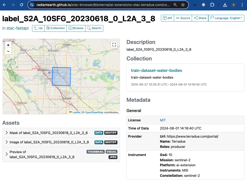
- Search STAC Item(s) on STAC endpoint with standard query params such as bbox and time range, but also ML-specific params such as model architecture or hyperparameters.
Practical examples and commands are displayed to demonstrate how these new capabilities can be used from a Jupyter Notebook.
Create / Upload STAC Objects
This section allows the user to either:
- Create a STAC Item using
pystac, or:
- Upload an existing STAC Item (
.json/.geojson file)
Create STAC Item
The STAC Item is create with pystac library with the following steps:
# Import Libraries
import pystac

# Create STAC Item with key properties
item = pystac.Item(
   id='water-bodies-model-pystac',
   bbox=bbox,
   geometry=getGeom(bbox),
   datetime=datetime.now(),
   properties={
      "start_datetime": "2024-06-13T00:00:00Z"
      "end_datetime": "2024-07-13T00:00:00Z"
      "description": "Water bodies classifier with Scikit-Learn Random-Forest"
   }
)
Add relevant STAC Extensions using their latest references, below:
from pystac.extensions.eo import EOExtension

# Add Extensions
EOExtension.ext(item, add_if_missing=True)
item.stac_extensions.append('https://stac-extensions.github.io/ml-model/v1.0.0/schema.json')
item.stac_extensions.append('https://crim-ca.github.io/mlm-extension/v1.2.0/schema.json')
item.stac_extensions.append("https://stac-extensions.github.io/raster/v1.1.0/schema.json")
item.stac_extensions.append("https://stac-extensions.github.io/file/v2.1.0/schema.json")
Add ml-model properties
# Add "ml-model" properties
item.properties["ml-model:type"] = "ml-model"
item.properties["ml-model:learning_approach"] = "supervised"
item.properties["ml-model:prediction_type"] = "segmentation"
item.properties["ml-model:architecture"] = "RandomForestClassifier"
item.properties["ml-model:training-processor-type"] = "cpu"
item.properties["ml-model:training-os"] = "linux"
Add mlm-extension properties
# Add "mlm-extension" properties
item.properties["mlm:name"] = "Water-Bodies-S6_Scikit-Learn-RandomForestClassifier"
item.properties["mlm:architecture"] = "RandomForestClassifier"
item.properties["mlm:framework"] = "scikit-learn"
item.properties["mlm:framework_version"] = "1.4.2"
item.properties["mlm:tasks"] = [
      "segmentation",
      "semantic-segmentation"
    ]
item.properties["mlm:pretrained_source"] = None
item.properties["mlm:compiled"] = False
item.properties["mlm:accelerator"] = "amd64"
item.properties["mlm:accelerator_constrained"] = True

# Add hyperparameters
item.properties["mlm:hyperparameters"] = {
  "bootstrap": True,
  "ccp_alpha": 0.0,
  "class_weight": None,
  "criterion": "gini",
  "max_depth": None,
  "max_features": "sqrt",
  "max_leaf_nodes": None,
  "max_samples": None,
  "min_impurity_decrease": 0.0,
  "min_samples_leaf": 1,
  "min_samples_split": 2,
  "min_weight_fraction_leaf": 0.0,
  "monotonic_cst": None,
  "n_estimators": 200,
  "n_jobs": -1,
  "oob_score": False,
  "random_state": 19,
  "verbose": 0,
  "warm_start": True
  }
Add input and output to the mlm properties
# Add input and output to the properties
item.properties["mlm:input"] = [
{
"name": "EO Data",
"bands": ["B01","B02","B03","B04","B08","B8A","B09","B11","B12","NDVI","NDWI1","NDWI2"],
"input": {
"shape": [-1,12,10980,10980],
"dim_order": ["batch","channel","height","width"],
"data_type": "float32"
},
"norm_type": None,
"resize_type": None,
"pre_processing_function": None
}
]
item.properties["mlm:output"] = [
{
"name": "CLASSIFICATION",
"tasks": ["segmentation","semantic-segmentation"],
"result": {
"shape": [-1,10980,10980],
"dim_order": ["batch","height","width"],
"data_type": "uint8"
},
"post_processing_function": None,
"classification:classes": [
{
"name": "NON-WATER",
"value": 0,
"description": "pixels without water",
"color_hint": "000000",
"nodata": False
},
{
"name": "WATER",
"value": 1,
"description": "pixels with water",
"color_hint": "0000FF",
"nodata": False
},
{
"name": "CLOUD",
"value": 2,
"description": "pixels with cloud",
"color_hint": "FFFFFF",
"nodata": False
}
]
}
]
Add raster:bands properties, which can be either standard EO bands as well calculated from expressions, for example to calculate vegetation indices. Both examples are given below.
item.properties["raster:bands"] = [
    {
        "name": "B01",
        "common_name": "coastal",
        "nodata": 0,
        "data_type": "uint16",
        "bits_per_sample": 15,
        "spatial_resolution": 60,
        "scale": 0.0001,
        "offset": 0,
        "unit": “m”
    },
    ...,
    {
        "name": NDVI,
        "common_name": ndvi,
        "nodata": 0,
        "data_type": float32,
        "processing:expression": {
            "format": "rio-calc",
            "expression": "(B08 - B04) / (B08 + B04)"
        }
    }
Now the user can add the assets to the STAC Item of the ML model. The required assets are:
- Asset for App Package CWL for ML Training
- Asset for App Package CWL for Inference
- Asset for ML Model (i.e.
.onnx file)
# Add Assets - ML Training
asset = pystac.Asset(
    title='Workflow for water bodies training',
    href='https://github.com/ai-extensions/notebooks/releases/download/v1.0.8/water-bodies-app-training.1.0.8.cwl',
    media_type='application/cwl+yaml',
    roles = ['ml-model:training-runtime', 'runtime', 'mlm:training-runtime'])
item.add_asset("ml-training", asset)

# Add Assets - Inference
asset = pystac.Asset(
    title='Workflow for water bodies inference',
    href='https://github.com/ai-extensions/notebooks/releases/download/v1.0.8/water-bodies-app-inference.1.0.8.cwl',
    media_type='application/cwl+yaml',
    roles = ['ml-model:inference-runtime', 'runtime', 'mlm:inference-runtime'])
item.add_asset("ml-inference", asset)

# Add Asset - ML model
asset = pystac.Asset(
    title='ONNX Model',
    href='https://github.com/ai-extensions/notebooks/raw/main/scenario-7/model/best_model.onnx',
    media_type='application/octet-stream; framework=onnx; profile=onnx',
    roles = ['mlm:model'])
item.add_asset("model", asset)
Now the created STAC Item can be validated.
item.validate()

Output of successful validation:
['https://schemas.stacspec.org/v1.0.0/item-spec/json-schema/item.json',
 'https://stac-extensions.github.io/eo/v1.1.0/schema.json',
 'https://stac-extensions.github.io/ml-model/v1.0.0/schema.json',
 'https://crim-ca.github.io/mlm-extension/v1.2.0/schema.json',
 'https://stac-extensions.github.io/raster/v1.1.0/schema.json',
 'https://stac-extensions.github.io/file/v2.1.0/schema.json']
Upload STAC Item
If the user has manually written a .json / .geojson file of the STAC Item, this can be simply uploaded into the notebook with pystac. The Item can subsequently be validated as it was done before.
# Read Item
item = pystac.read_file('./path/to/STAC_Item.json')

# Validate STAC Item
item.validate()

Output of successful validation:
['https://schemas.stacspec.org/v1.0.0/item-spec/json-schema/item.json',
 'https://stac-extensions.github.io/eo/v1.1.0/schema.json',
 'https://stac-extensions.github.io/ml-model/v1.0.0/schema.json',
 'https://crim-ca.github.io/mlm-extension/v1.2.0/schema.json',
 'https://stac-extensions.github.io/raster/v1.1.0/schema.json',
 'https://stac-extensions.github.io/file/v2.1.0/schema.json']
STAC Objects
The STAC Catalog and STAC Collection need to be created and interlinked with each other and the STAC Item (see related Article dedicated to STAC for more information about the STAC format).
Create STAC Catalog
# Create folder structure
CAT_DIR = "ML_Catalog"
COLL_NAME = "ML-Models"
SUB_DIR = os.path.join(CAT_DIR,COLL_NAME)

# Create Catalog
catalog = pystac.Catalog(
    id = "ML-Models",
    description = "A catalog to describe ML models",
    title="ML Models"
)
Create STAC Collection
collection = pystac.Collection(
    id = COLL_NAME,
    description = "A collection for ML Models",
    extent = pystac.Extent(
        spatial=<spatial_extent>,
        temporal=<temporal_extent>
    ),
    title = COLL_NAME,
    license = "properietary",
    keywords = [],
    stac_extensions=["https://schemas.stacspec.org/v1.0.0/collection-spec/json-schema/collection.json"],
    providers=[
        pystac.Provider(
            name = "AI-Extensions Project",
            roles = ["producer"],
            url = "https://ai-extensions.github.io/docs"
        )
    ]
)
Now the user can create the interlinks between STAC Catalog, STAC Collection and STAC Item
# Add STAC Item to the Collection
collection.add_item(item=item)

# Add Collection to the Catalog
catalog.add_child(collection)
Finally, the user can normalise and save locally the three STAC Objects and then check that these have been created successfully, using the dedicated pystac methods
# Save STAC Objects to files
catalog.normalize_and_save(root_href=CAT_DIR,
                           catalog_type=pystac.CatalogType.SELF_CONTAINED)


# Check that the STAC Catalog contains the Collection, and the Collection contains the Item
catalog.describe()

Example output:
* <Catalog id=ML-Models>
    * <Collection id=ML-Models>
      * <Item id=water-bodies-model-pystac>
Post on S3 bucket
Once the STAC Objects are created, they can be posted on the AWS S3 bucket. A custom class is defined using the pystac, boto3 and botocore libraries to interact with S3. This class allows configuring access to a specific bucket using pre-defined user settings in the development environment ML Lab, including endpoint, access key credentials, and other related settings.
# Import libraries
from pystac.stac_io import DefaultStacIO, StacIO
import boto3, import botocore

# Create S3 client object
bucket_name = 'my_bucket'
settings = UserSettings("/etc/Stars/appsettings.json")
settings.set_s3_environment(f"s3://{bucket_name}/{SUB_DIR}")
StacIO.set_default(DefaultStacIO)
client = boto3.client(
    service_name="s3",
    region_name=os.environ.get("AWS_REGION"),
    use_ssl=True,
    endpoint_url=os.environ.get("AWS_S3_ENDPOINT"),
    aws_access_key_id=os.environ.get("AWS_ACCESS_KEY_ID"),
    aws_secret_access_key=os.environ.get("AWS_SECRET_ACCESS_KEY"),
)

# Configure and set custom Class
class CustomStacIOs(DefaultStacIO):
    """Custom STAC IO class that uses boto3 to read from S3."""

    def __init__(self):
        self.session = botocore.session.Session()
        self.s3_client = self.session.create_client(
            service_name="s3",
            region_name=os.environ.get("AWS_REGION"),
            use_ssl=True,
            endpoint_url=os.environ.get("AWS_S3_ENDPOINT"),
            aws_access_key_id=os.environ.get("AWS_ACCESS_KEY_ID"),
            aws_secret_access_key=os.environ.get("AWS_SECRET_ACCESS_KEY"),
        )

    def write_text(self, dest, txt, *args, **kwargs):
        parsed = urlparse(dest)
        if parsed.scheme == "s3":
            self.s3_client.put_object(
                Body=txt.encode("UTF-8"),
                Bucket=parsed.netloc,
                Key=parsed.path[1:],
                ContentType="application/geo+json",
            )
        else:
            super().write_text(dest, txt, *args, **kwargs)
StacIO.set_default(CustomStacIOs)
The user also makes use of the concurrent.futures and tqdm libraries. The former allows running tasks asynchronously managing multiple threads or processes in parallel. The latter is used to monitor and understand progress of a running process.
# Import libraries
import concurrent.futures
from concurrent.futures import ProcessPoolExecutor,ThreadPoolExecutor
from tqdm import tqdm


# push assets and STAC objs to s3
def upload_asset(item, key, asset, SUB_DIR):
    s3_path = os.path.normpath(
        os.path.join(os.path.join(SUB_DIR, SUB_DIR, item.id, asset.href))
    )
    item.add_asset(key, asset)

futures = []
with concurrent.futures.ThreadPoolExecutor(max_workers=4) as executor:
    for item in tqdm(items):
        for key, asset in item.assets.items():
            future = executor.submit(upload_asset, item, key, asset, SUB_DIR)
            futures.append(future)


    # Wait for all uploads to complete
    for _ in tqdm(concurrent.futures.as_completed(futures), total=len(futures), desc="Uploading"):
        pass
Post STAC Objects to S3
# Update STAC Catalog with new urls point to S3
catalog.set_root(catalog)
catalog.normalize_hrefs(f"s3://{bucket_name}/{SUB_DIR}")
items = list(tqdm(catalog.get_all_items()))

# push STAC Item(s) to S3 in parallel
futures = []
def write_and_upload_item(client, item, bucket_name):
    # Write STAC item to file
    s3_path = item.get_self_href()
    pystac.write_file(item, item.get_self_href())

with concurrent.futures.ThreadPoolExecutor(max_workers=4) as execute:
    for item in tqdm(items, desc="Processing Items"):
        future = execute.submit(write_and_upload_item,client ,item, bucket_name)
        futures.append(future)

    # Wait for all processes to complete
    for _ in tqdm(concurrent.futures.as_completed(futures), total=len(futures), desc="Uploading Items"):
        pass

# push STAC Collection to S3
for col in tqdm(catalog.get_all_collections(),desc="Processing Collection"):
    pystac.write_file(col, col.get_self_href())

# push STAC Catalog to S3
pystac.write_file(catalog, catalog.get_self_href())
print("STAC Objects are pushed successfully")
An example of output log is shown below
100%|██████████| 2/2 [00:00<00:00, 266.00it/s]
Uploading: 100%|██████████| 5/5 [00:00<00:00, 59409.41it/s]
2it [00:00, 22610.80it/s]
Processing Items: 100%|██████████| 2/2 [00:00<00:00, 78.49it/s]
Uploading Items: 100%|██████████| 2/2 [00:00<00:00,  3.06it/s]
Processing Collection: 1it [00:00,  1.24it/s]
STAC Objects are pushed successfully
Publish on STAC endpoint
Now that the STAC Objects are posted on S3, the user can publish them on the STAC endpoint with the code below.
# Define STAC endpoint
stac_endpoint = "https://ai-extensions-stac.terradue.com"

# Create a new Collection on the endpoint
from urllib.parse import urljoin
def post_or_put(url: str, data, headers=None): # function to post/put STAC obj to the endpoint using REST API
    if headers is None:
        headers = get_headers()
    try:
        request = requests.post(url, json=data, timeout=20, headers=headers)

    # Print or log the content of the response
    except:
        new_url = url if data["type"] == "Collection" else f"{url}/{data['id']}"
        request = requests.put(new_url, json=data, timeout=20, headers=headers)
    return request

response = post_or_put(urljoin(stac_endpoint, "/collections"),
   collection.to_dict(),
   headers=get_headers())
if response.status_code == 200: print(f"Collection {collection.id} created successfully")
else: print(f"ERROR: Collection {collection.id} exists already, please check")

# Set custom Class and read the STAC Catalog posted on S3
StacIO.set_default(CustomStacIO)

catalog_s3 = read_url(catalog.self_href)

# Run function to publish STAC Item(s) in STAC endpoint
ingest_items(
    app_host=stac_endpoint,
    items=list(catalog_s3.get_all_items()),
    collection=collection,
    headers=get_headers(),
)
An example of output log is shown below
2024-07-26 08:02:43.961 | INFO     | utils:ingest_items:187 - Post item water-bodies-model-pystac to https://ai-extensions-stac.terradue.com/collections/ML-Models/items
https://ai-extensions-stac.terradue.com/collections/ML-Models/items/water-bodies-model-pystac
Discover ML Model with STAC
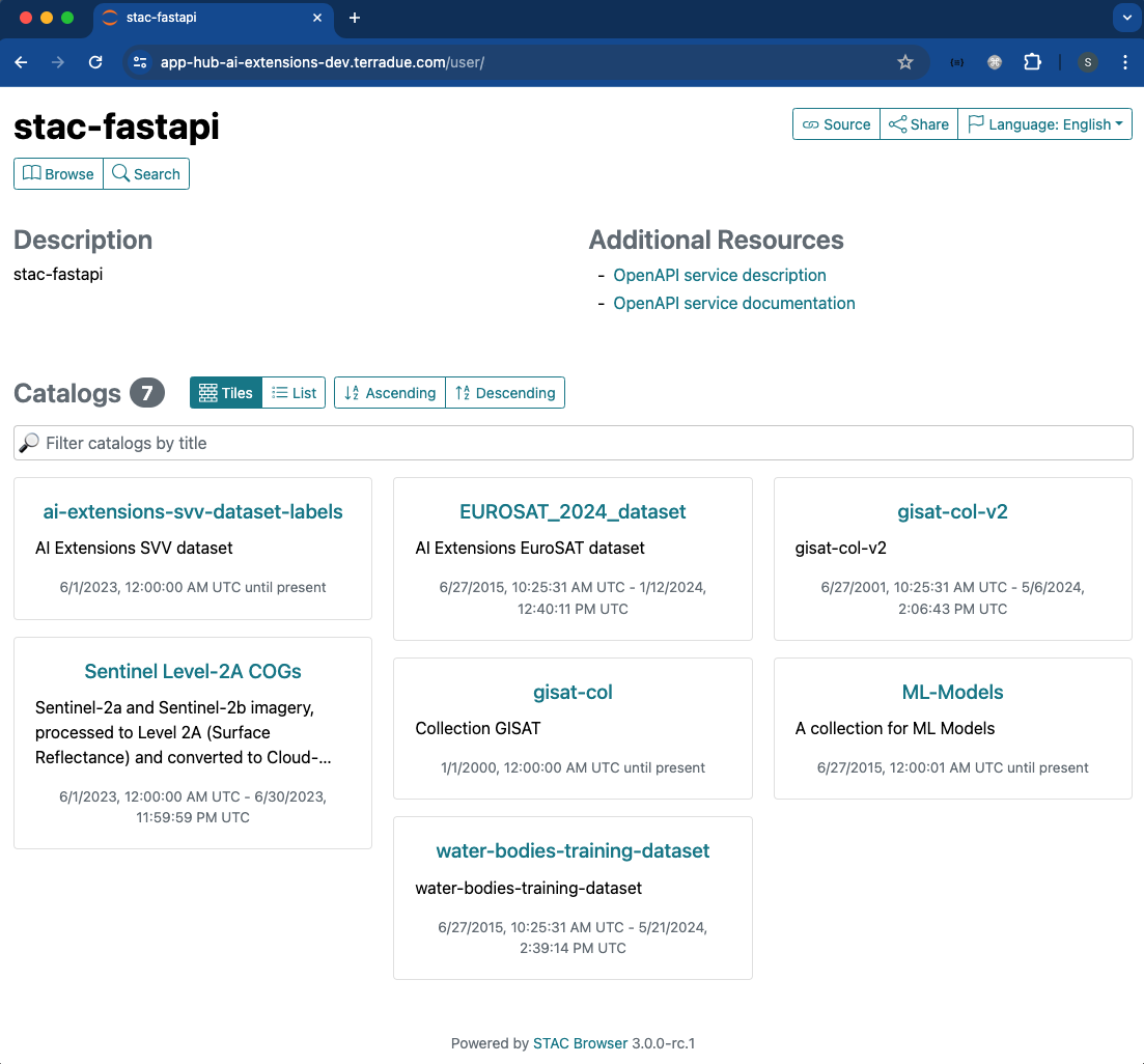
Once the STAC Objects are posted on S3 and on the STAC endpoint successfully, the user can perform a search on such STAC endpoint using specific query parameters. Only the STAC Item(s) that align with the provided criteria is(are) retrieved for the user. This can be achieved with the pystac and pystac_client libraries.
# Import libraries
import pystac
from pystac_client import Client

# Define STAC endpoint and access to the Catalog
stac_endpoint = "https://ai-extensions-stac.terradue.com"
cat = Client.open(stac_endpoint, headers=get_headers(), ignore_conformance=True)

# Define date
start_date = datetime.strptime('20230614', '%Y%m%d')
end_date = datetime.strptime('20230620', '%Y%m%d')
date_time = (start_date, end_date)

# Define bbox
bbox = [-121.857043 ,  37.853934 ,-120.608968  , 38.840424]

query = {
    # `ml-model` properties
    "ml-model:prediction_type": {"eq": 'segmentation'},
    "ml-model:architecture": {"eq": "RandomForestClassifier"},
    "ml-model:training-processor-type": {"eq": "cpu"},

    # `mlm-model` properties
    "mlm:architecture": {"eq": "RandomForestClassifier"},
    "mlm:framework": {"eq": "scikit-learn"},
    "mlm:hyperparameters.random_state": {"gt": 18},
    "mlm:compiled": {"eq": False},
    "mlm:hyperparameters.bootstrap": {"eq": True}
    }

# Query by AOI, TOI and ML-specific params
query_sel = cat.search(
    collections= collection,
    datetime=date_time,
    bbox=bbox,
    query = query
)
items = [item for item in query_sel.item_collection()]
For the example query above, the following items were retrieved:
[<Item id=water-bodies-model-pystac>,
 <Item id=water-bodies-model>]
Conclusion
This work demonstrates the new functionalities brought by the AI/ML Enhancement Project to support a ML practitioner on describing an ML model using the STAC format. The activities covered are listed below:
- Create a STAC Item, either with
pystac or by uploading an existing STAC Item into the Notebook, and its related Catalog and Collection. The STAC Item contains all related ML model specific properties, related STAC extensions and hyperparameters.
- Post STAC Objects onto S3 bucket
- Publish STAC Objects onto STAC endpoint
- Search STAC Item(s) on STAC endpoint with standard query params such as bbox and time range, but also ML-specific params such as model architecture or hyperparameters.
Useful links: