AI/ML Enhancement Project - Developing a new ML model and tracking with MLflow
Introduction
In this scenario, the ML practitioner Alice develops a Convolutional Neural Networks (CNN) model for a classification task and employs MLflow for monitoring the ML model development cycle. MLflow is a crucial tool that ensures effective log tracking and preserves key information, including specific code versions, datasets used, and model hyperparameters. By logging this information, the reproducibility of the work drastically increases, enabling users to revisit and replicate past experiments accurately. Moreover, quality metrics such as classification accuracy, loss function fluctuations, and inference time are also tracked, enabling easy comparison between different models.
This post presents User Scenario 5 of the AI/ML Enhancement Project, titled “Alice develops a new ML model”. It demonstrates how the enhancements being deployed in the Geohazards Exploitation Platform (GEP) and Urban Thematic Exploitation Platform (U-TEP) will support users on developing a new ML model and on using MLflow to track experiments.
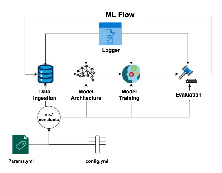
These new capabilities are implemented with an interactive Jupyter Notebook to guide an ML practitioner, such as Alice, through the following steps:
- Data ingestion
- Design the ML model architecture
- Train the ML model and fine-tuning
- Evaluate the ML model performance with metrics such as accuracy, precision, recall, or F1 score, and confusion matrix
- Check experiments with MLflow
These steps are outlined in the diagram below.
Practical examples and commands are displayed to demonstrate how these new capabilities can be used from a Jupyter Notebook.
Data Ingestion
The training data used for this scenario is the EuroSAT dataset. The EuroSAT dataset is based on ESA’s Sentinel-2 data, covering 13 spectral bands and consisting out of 10 classes with a total of 27,000 labelled and geo-referenced images. A separate Notebook was generated to create a STAC Catalog, a STAC Collection, and STAC Items for the entire EuroSAT dataset, and then publish these into the STAC endpoint (https://ai-extensions-stac.terradue.com/collections/EUROSAT-Training-Dataset).
The data ingestion process was implemented with a DataIngestion class, configured with three main components:
stac_loader: for fetching the dataset from the STAC endpointdata_splitting: for splitting the dataset intotrain,testandvalidationsets with defined percentagesdata_downloader: for downloading the data into the local system.
ML Model Architecture
In this section, the user defines a Convolutional Neural Networks (CNNs) model with six layers. The first layer serves as the input layer, accepting an image with a defined shape of (13, 64, 64) (i.e. same as the shape of the EuroSAT labels in this case). The model is designed with four convolutional layers, each employing: a relu activation function, a BatchNormalization layer, a 2D MaxPooling operation, and a Dropout layer. Subsequently, the model includes two Dense layers and finally, a Softmax activation layer is implied in the last Dense layer which generates a vector with 10 cells containing the likelihood of the predicted classes. The user defines a loss function and an optimizer, and eventually the best model is compiled and saved locally for each epoch based on the improvement in validation loss function. The input parameters defining the ML model architecture are described in a params.yml file which is used for the configuration process. See below for the params.yml file defined in this test.
params.yml
BATCH_SIZE: 128
EPOCHS: 50
LEARNING_RATE: 0.001
DECAY: 0.1 ### float
EPSILON: 0.0000001
MEMENTUM: 0.9
LOSS: categorical_crossentropy
# choose one of l1,l2,None
REGULIZER: None
OPTIMIZER: SGD
The configuration of the ML model architecture is run with a dedicated pipeline, such as that defined below.
# pipeline
try:
  config = ConfigurationManager()
  prepare_base_model_config = config.get_prepare_base_model_config()
  prepare_base_model = PrepareBaseModel(config=prepare_base_model_config)
  prepare_base_model.base_model()
except Exception as e:
  raise e
The output of the ML model architecture configuration is displayed below, allowing the user to summarise the model and report the number of trainable and non-trainable parameters.
Model: "sequential"
___________________________________________________________________
 Layer (type)                    Output Shape              Param #
===================================================================
 conv2d (Conv2D)                 (None, 64, 64, 32)        3776
 activation (Activation)         (None, 64, 64, 32)        0
 conv2d_1 (Conv2D)               (None, 62, 62, 32)        9248
 activation_1 (Activation)       (None, 62, 62, 32)        0
 max_pooling2d (MaxPooling2D)    (None, 31, 31, 32)        0
 dropout (Dropout)               (None, 31, 31, 32)        0
 conv2d_2 (Conv2D)               (None, 31, 31, 64)        18496
 activation_2 (Activation)       (None, 31, 31, 64)        0
 conv2d_3 (Conv2D)               (None, 29, 29, 64)        36928
 activation_3 (Activation)       (None, 29, 29, 64)        0
 max_pooling2d_1 (MaxPooling2D)  (None, 14, 14, 64)        0
 dropout_1 (Dropout)             (None, 14, 14, 64)        0
 flatten (Flatten)               (None, 12544)             0
 dense (Dense)                   (None, 512)               6423040
 activation_4 (Activation)       (None, 512)               0
 dropout_2 (Dropout)             (None, 512)               0
 dense_1 (Dense)                 (None, 10)                5130
 activation_5 (Activation)       (None, 10)                0
===================================================================
Total params: 6,496,618
Trainable params: 6,496,618
Non-trainable params: 0
===================================================================
Training and fine-tuning
The steps involved in the training phase are as follows:
- Create the training entity
- Create the configuration manager
- Define the training component
- Run the training pipeline
As mentioned in the “Training Data Ingestion” chapter, the training data was split into train, test and validation sets in order to ensure that the model is trained effectively and its performance is evaluated accurately and without bias. The user trains the ML model on the train data set for a specific number of epochs, defined in the params.yml file, after each epoch the model is evaluated on the validation data to avoid overfitting. There are several approaches to address overfitting during training. One effective method is adding a regularizer to the model’s layers, which introduces a penalty term to the loss function to penalize larger weights. In the end, the test set, which is not used in any part of the training or validation process, is used to evaluate the final model’s performance.
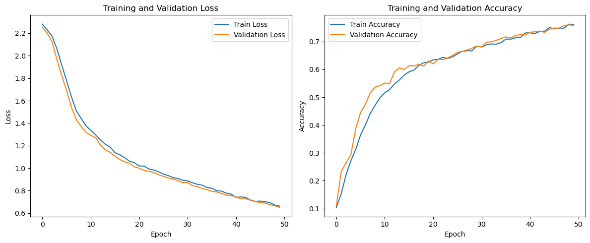
In order to assess the ML model’s performance and reliability, the user can plot the Loss and Accuracy curves of the Training and Validation sets. This can be done with the matplotlib library, as illustrated below.
# Import library
import matplotlib.pyplot as plt
plt.figure(figsize=(12, 5))

# Plot Loss
plt.subplot(1, 2, 1)
plt.plot(history.history['loss'], label='Train Loss')
plt.plot(history.history['val_loss'], label='Validation Loss')
plt.xlabel('Epoch')
plt.ylabel('Loss')
plt.title('Training and Validation Loss')
plt.legend()

# Plot Accuracy
plt.subplot(1, 2, 2)
plt.plot(history.history['accuracy'], label='Train Accuracy')
plt.plot(history.history['val_accuracy'], label='Validation Accuracy')
plt.xlabel('Epoch')
plt.ylabel('Accuracy')
plt.title('Training and Validation Accuracy')
plt.legend()
plt.tight_layout()
plt.show()
Evaluation
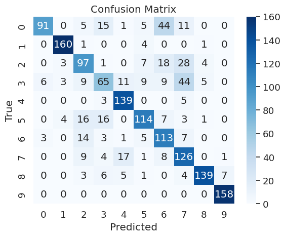
The evaluation of the trained ML model was conducted on the test set. It is crucial for the user to prevent any data leakage between the train and test sets to ensure an independent and unbiased assessment of the training pipeline’s outcome. The model’s performance was measured using the following evaluation metrics: accuracy, recall, precision, F1-score, and the confusion matrix.
- Accuracy: calculated as the ratio of correctly predicted instances to the total number of instances in the dataset
- Recall: also known as sensitivity or true positive rate, recall is a metric that evaluates the ability of a classification model to correctly identify all relevant instances from a dataset
- Precision: it evaluates the accuracy of the positive predictions made by a classification model
- F1-score: it is a metric that combines precision and recall into a single value. It is particularly useful when there is an uneven class distribution (imbalanced classes) and provides a balance between precision and recall
- Confusion Matrix: it provides a detailed breakdown of the model’s performance, highlighting instances of correct and incorrect predictions.
The pipeline for generating the evaluation metrics was defined as follows:
try:
  config = ConfigurationManager()
  eval_config = config.get_evaluation_config()
  evaluation = Evaluation(eval_config)
  test_dataset,conf_mat = evaluation.evaluation()
  evaluation.log_into_mlflow()
except Exception as e:
  raise e
The confusion matrix can be easily plotted with the seaborne library.
# Import libraries
import matplotlib.pyplot as plt
import seaborn as sn
import numpy as np
def plot_confusion_matrix(self):
  class_names = np.unique(self.y_true)
  fig, ax = plt.subplots()

  # Create a heatmap
  sns.heatmap(
    self.matrix,
    annot=True,
    fmt="d",
    cmap="Blues",
    xticklabels=class_names,
    yticklabels=class_names
  )

  # Add labels and title
  plt.xlabel('Predicted')
  plt.ylabel('True')
  plt.title('Confusion Matrix')
  # Show the plot
  plt.show()
MLflow Tracking
The training, fine-tuning, and evaluation processes are executed multiple times, referred to as “runs”. Each run is generated by executing multiple jobs with different combinations of parameters, specified in the params.yaml file described in the ML Model Architecture section. The user monitors all executed runs during the training and evaluation phases using mlflow and its built-in tracking functionalities, as shown in the code below.
# Import libraries
import mlflow
import tensorflow

def log_into_mlflow(self):
  mlflow.set_tracking_uri(os.environ.get("MLFLOW_TRACKING_URI"))
  tracking_url_type_store = urlparse(os.environ.get("MLFLOW_TRACKING_URI")).scheme
  confusion_matrix_figure = self.plot_confusion_matrix()

  with mlflow.start_run():
    mlflow.tensorflow.autolog()
    mlflow.log_params(self.config.all_params)
    mlflow.log_figure(confusion_matrix_figure, artifact_file="Confusion_Matrix.png")
    mlflow.log_metrics(
      {
        "loss": self.score[0], "test_accuracy": self.score[1],
        "test_precision":self.score[2],"test_recall":self.score[3],
      }
    )
    # Model registry does not work with file store
    if tracking_url_type_store != "file":
      log_model(self.model, "model", registered_model_name=f"CNN")
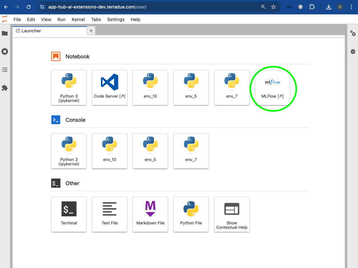
The MLflow dashboard allows for visual and interactive comparisons of different runs, enabling the user to make informed decisions when selecting the best model. The user can access the MLflow dashboard by clicking on the dedicated icon from the user’s App Hub dashboard.
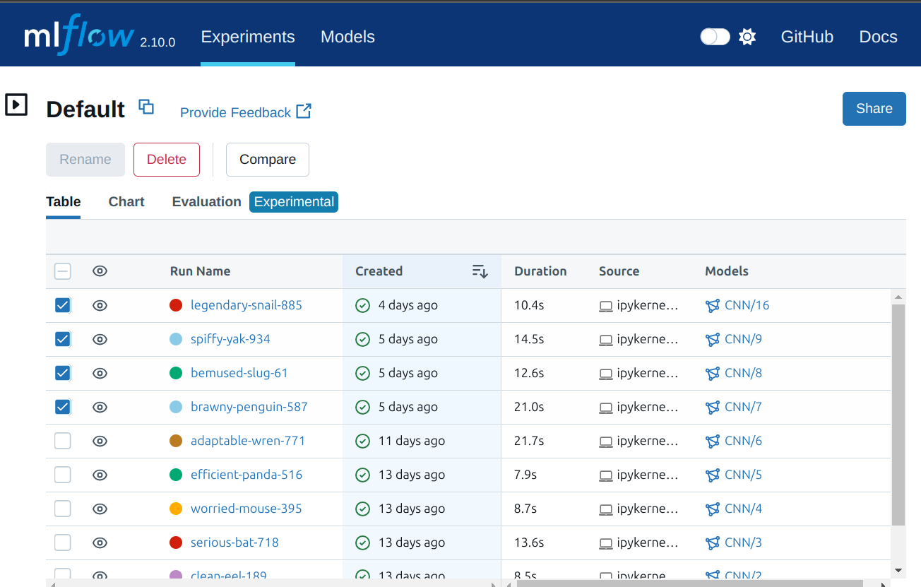
On the MLflow dashboard, the user can select the experiments to compare in the “Experiment” tab.
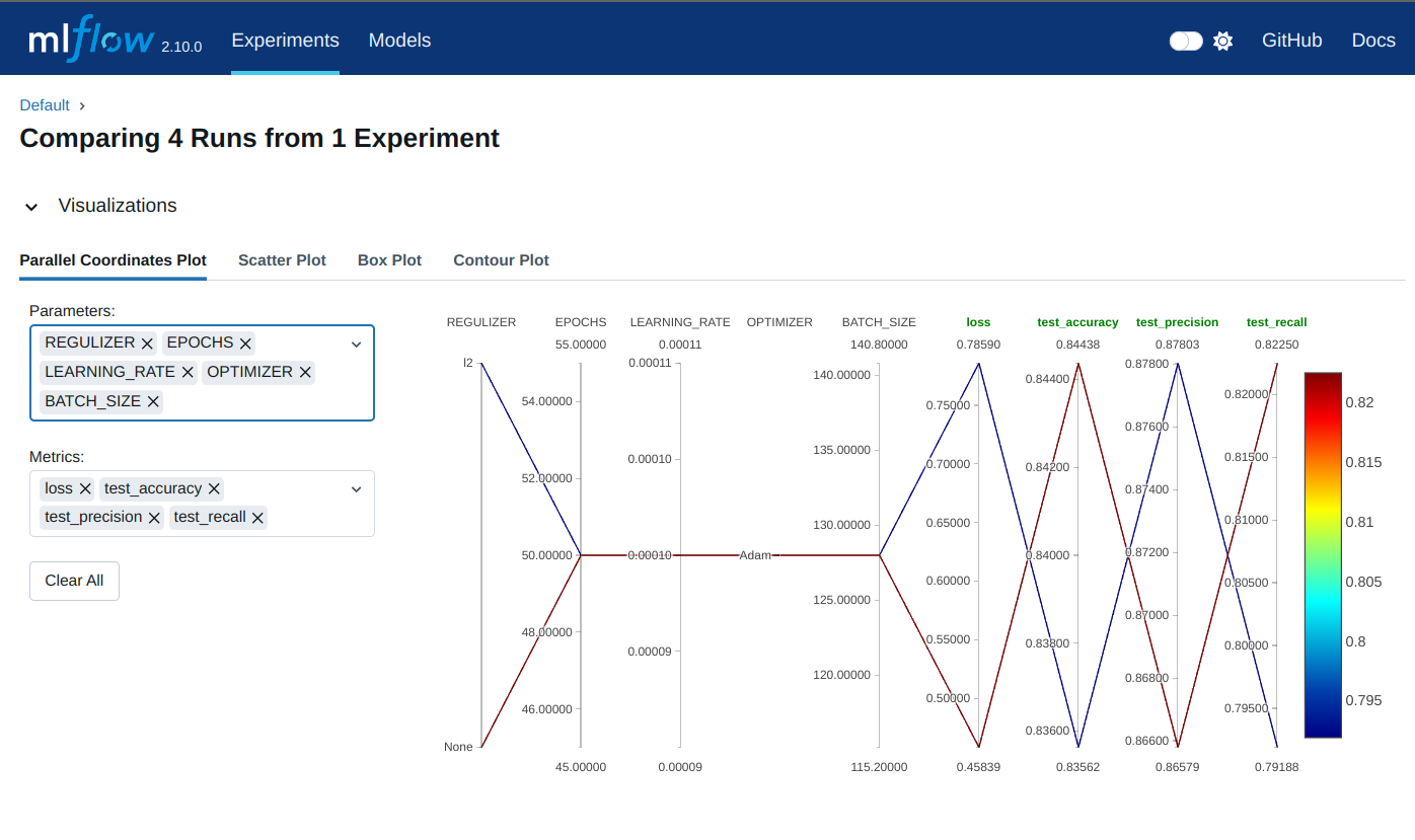
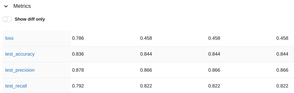
Subsequently, the user can select the specific parameters and metrics to include in the comparison from the “Visualizations” dropdown. The runs’ behavior and details generated by the different evaluation metrics and parameters are displayed.
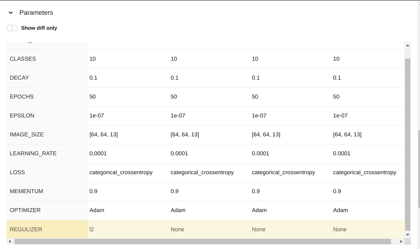
The comparison of the parameters and metrics are shown in the dedicated dropdown.
Conclusion
This work demonstrates the new functionalities brought by the AI/ML Enhancement Project to guide a ML practitioner through the development of a new ML model and its related tracking functionalities provided by MLflow, including:
- Data ingestion
- Design the ML model architecture
- Train the ML model and fine-tuning
- Evaluate the ML model performance with metrics such as accuracy, precision, recall, or F1 score, and confusion matrix
- Check experiments with MLflow dashboard and tools.
Useful links:
- The link to the Notebook for User Scenario 5 is: https://github.com/ai-extensions/notebooks/blob/main/scenario-5/trials/s5-newMLModel.ipynb
Note: access to this Notebook must be granted - please send an email to support@terradue.com with subject “Request Access to s5-newMLModel ” and body “Please provide access to Notebook for AI Extensions User Scenario 5” - The user manual of the AI/ML Enhancement Project Platform is available at AI-Extensions Application Hub - User Manual
- Project Update “AI/ML Enhancement Project - Progress Update”
- User Scenario 1 “AI/ML Enhancement Project - Exploratory Data Analysis”
- User Scenario 2 “AI/ML Enhancement Project - Labelling EO Data”
- User Scenario 3 “AI/ML Enhancement Project - Describing labelled EO data”
- User Scenario 4 “AI/ML Enhancement Project - Discovering labelled EO data with STAC”