AI/ML Enhancement Project - Reusing an existing pre-trained model
Introduction
In this scenario, the ML practitioner Alice reuses a pre-trained model by leveraging the power of transfer learning. Transfer learning, a widely adopted technique in deep learning, involves using an existing model, pre-trained on a large dataset, to train a new model on a smaller, task-specific dataset. This approach allows the new model to utilise the features learned by the pre-trained model, enabling it to extract valuable information from the input data more efficiently. Consequently, the new model can achieve higher accuracy even with limited data.
This post presents User Scenario 8 of the AI/ML Enhancement Project, titled “Alice reuses an existing pre-trained ML model”. It demonstrates how the enhancements being deployed in the Geohazards Exploitation Platform (GEP) and Urban Thematic Exploitation Platform (U-TEP) will support users on performing a semantic segmentation task with transfer learning in the context of Earth Observation (EO). This also includes the option to leverage the GPU resources set-up in the dedicated App Hub environment, significantly reducing the execution time for the model fine-tuning phase.
These new capabilities are implemented with an interactive Jupyter Notebook to guide an ML practitioner, such as Alice, through the following steps:
- Import libraries (e.g.
torch,sklearn,albumentation) - Data acquisition, including EO data search and data loader implementing different augmentation techniques (e.g.,
RandomCrop,Resize, andRandomRotate90) and data loading in batches - Data visualization to enable the user to gain comprehensive insights of data distribution
- Selection of pre-trained ML model, in this case with a
UNetbackbone trained onImageNet, and subsequently implementation of fine-tuning adjustments - Evaluation of outputs using different techniques on unseen dataset (e.g., plotting
lossfunctions, calculatingmIoU) - Inference on the unseen
testdataset.
Practical examples and commands are displayed to demonstrate how these new capabilities can be used from a Jupyter Notebook.

Key Python Libraries
Three key Python libraries were used for this scenario: PyTorch, segmentation_models, and albumentations:
PyTorch: This deep learning framework is well-suited for transfer learning in the context of EO semantic segmentation due to its flexibility and extensive support for deep learning models. It is widely used in academia, and research paper’s code written withpytorchare often available on Github for reproducibility purposes.segmentation_models: Built onPyTorch, this library provides pre-trained models tailored for various segmentation tasks, significantly reducing training time.albumentations: This library constructs data augmentation pipelines, enriching the training dataset and generalisation of trained models.
These libraries work together seamlessly within the PyTorch ecosystem, enabling the user to utilise other tools like TorchMetrics for improved model performance evaluation.
Note: In order to leverage the GPU resources and make the most of these libraries, the user must switch to the dedicated profile on the ML Lab environment. This can be done with the following steps:
- Stop the current pod by going on https://app-hub-ai-extensions-dev.terradue.com/hub/user/
- Select Home > Stop my Server
- Select Start my Server
- Select the Machine Learning Lab with GPU vX.Y profile and click Start
Data Acquisition Pipeline
Data Acquisition
The candidate dataset for this task was OpenEarthMap, which is a benchmark dataset for global high-resolution land cover mapping. It consists of 5000 aerial and satellite images with manually annotated 8-class land cover labels and 2.2 million segments at a 0.25-0.5m ground sampling distance, covering 97 regions from 44 countries across 6 continents.
# Set-up dataset information
DATA_URLS = {"OpenEarthMap_wo_xBD":"https://zenodo.org/records/7223446/files/OpenEarthMap.zip?download=1"}
SELECTED_DATA = {
    "DATASET_NAME": "OpenEarthMap_wo_xBD",
    "DATA_URL" : DATA_URLS["OpenEarthMap_wo_xBD"] }
CLASSES = [
    "Bareland",
    "Rangeland",
    "Developed_Space",
    "Road",
    "Tree",
    "Water",
    "Agriculture_Land",
    "Building",
]
RANDOM_STATE = 17
BATCH_SIZE = 4
IMAGE_SIZE = 300
DEVICE = "cuda" if torch.cuda.is_available() else "cpu"

# Data Acquisition
data_obj = Acquisition(data_url=SELECTED_DATA['DATA_URL'],
                       data_file=SELECTED_DATA["DATASET_NAME"]+'.zip',
            source = "Gdrive")
data_obj.download_and_unzip_file()
data_obj.data_dir = SELECTED_DATA["DATASET_NAME"]
data_obj.check_and_remove_empty_regions()
data_obj.read_files()
sorted_image_list, sorted_mask_list = data_obj.sort_image_mask_files()
data_obj.check_if_sorted(sorted_image_list, sorted_mask_list)
Data Loader and Data Augmentation
Once the dataset was downloaded and locally accessible, a custom class MultiClassSegDataset, inheriting from the Dataset class, was created in PyTorch. This class reads training or evaluation images and ground truth masks from disk, and carries out transformations such as normalisation. Subsequently, the user split the data into train, validation, and test datasets with ratios of 80%, 10%, and 10%, respectively. The training set is used for model training, the validation set for model selection, and the test set for assessing the model’s generalisation error on unseen images.
Data augmentation was applied to artificially increase the number of training examples. This involved applying image transformations such as random cropping, rotation, and brightness adjustments while ensuring the corresponding mask remained aligned with the transformed image. It was crucial to select transformations that produced an augmented training set representative of the target application images. For the test set, a centered cropping operation was applied to maintain consistency in the comparative model performance evaluations and ensure reproducible outcomes. Conversely, random cropping was applied to the training set to generate diverse samples, helping the model learn from different image patches and improving its generalisation capability.
Some example code of these key concepts is shown below.
# Import libraries
from torch.utils.data import Dataset, DataLoader, Subset
from sklearn.model_selection import KFold, train_test_split
import albumentations as A

# Split data into train, val, test
train_images, test_images, train_masks, test_masks = train_test_split(sorted_image_list, sorted_mask_list, test_size=0.1, random_state=RANDOM_STATE)
train_images, valid_images, train_masks, valid_masks = train_test_split(train_images, train_masks, test_size=0.1, random_state=RANDOM_STATE)

# Define tranforms using Albumations
train_transform = A.Compose(
    [
        A.RandomCrop(IMAGE_SIZE, IMAGE_SIZE, always_apply=True),
        A.Resize(256, 256, always_apply=True),
        A.RandomRotate90(0.5)
    ]
)
test_transform = A.Compose(
    [
     A.CenterCrop(IMAGE_SIZE, IMAGE_SIZE, always_apply=True),
     A.Resize(256, 256, always_apply=True),
     ]
)

# Create the `MultiClassSegDataset` datasets
trainDS = MultiClassSegDataset(train_images, train_masks, classes=CLASSES, transform=train_transform)
validDS = MultiClassSegDataset(valid_images,valid_masks, classes=CLASSES, transform=test_transform)
testDS = MultiClassSegDataset(test_images,test_masks, classes=CLASSES, transform=test_transform)
Once the custom Datasets were created (trainDS, validDS, and testDS), the pytorch DataLoader class was used to provide an efficient and flexible way to iterate over a dataset, managing batching, shuffling, and parallel data loading. This class facilitates the application of different augmentation techniques (e.g., RandomCrop, Resize, and RandomRotate90) and the loading of the data in batches.
# Define DataLoaders
trainDL = DataLoader(trainDS,
                       batch_size=BATCH_SIZE,
                       shuffle=True,
                       num_workers=1,
                       pin_memory=True,
                       )
...

print(f"Number of Training Samples: {len(train_images)} \nNumber of Validation Samples: {len(valid_images)} \nNumber of Test Samples: {len(test_images)}")

# Printed Output:
Number of Training Samples: 577
Number of Validation Samples: 102
Number of Test Samples: 76
Data Visualisation
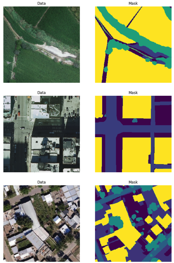
Before proceeding to model training, some data and their corresponding segmented masks were plotted to allow performing a sanity check by visually inspecting them. This helps identify any obvious data transformation mistakes or inconsistencies.
Model Selection for Transfer Learning
Transfer learning involves taking a pre-trained deep learning model, which has been trained on a large dataset (often on tasks like image classification with thousands of images), and adapting it to a new, typically smaller, dataset for a different but related task. In this scenario the pre-trained model was adapted for semantic segmentation, a task that involves classifying each pixel in an image.
Many deep learning computer vision models are pre-trained on datasets such as ImageNet, where the task is multi-class classification. By training on this dataset, the deep learning model (often using convolutional layers), learns to identify textures, geometric properties, shapes, and features from each image rather than reasoning on a pixel level. Transfer learning typically involves freezing these pre-trained layers, adding more layers (or unfreezing the last few layers), adapting the output layers to the desired task, and then continuing training.
ResNet is popular for image segmentation tasks due to its deep architecture with residual connections, which helps in effectively training very deep networks by mitigating the vanishing gradient problem. UNet, designed specifically for biomedical image segmentation, features a symmetric encoder-decoder structure with skip connections, enabling precise localization by combining high-level and low-level features. Both architectures have proven effective in various segmentation benchmarks, demonstrating high accuracy and robustness in diverse applications.
In this case, we leveraged the Unet architecture with a ResNet34 backbone and pre-trained weights from ImageNet for the encoder. The first layer was adjusted to accommodate the three input channels. Additionally, the final layer was updated to match the number of classes required for our target segmentation task.
# Import libraries
import torch
import segmentation_models_pytorch as smp

# Initiate UNet++ Model
MULTICLASS_MODE: str = "multiclass"
ENCODER = "resnet34"
ENCODER_WEIGHTS = "imagenet"
DECODER_ATTENTION_TYPE = None
EPOCHS = 50
ACTIVATION = None

model = smp.Unet(
    encoder_name=ENCODER,
    encoder_weights=ENCODER_WEIGHTS,
    in_channels=3,
    classes=9,
    activation=ACTIVATION
)
optimizer = torch.optim.Adam(
    [dict(params=model.parameters(), lr=0.0001)]
)
If the user is running the profile with GPU resources, the code below is used to check if multiple GPUs are available and, if so, enables certain CUDA backend features and prepares the model for parallel processing across these GPUs.
if torch.cuda.device_count() > 1:
    torch.backends.cudnn.enabled
    print("Number of GPUs :", torch.cuda.device_count())
    model = torch.nn.DataParallel(model)
Model Fine-tuning
The process involved modifying the architecture and hyperparameters of the selected pre-trained model ResNet to meet the specific requirements of the semantic segmentation task. After these adjustments, the model was trained and validated over a specified number of epochs (e.g., 50 epochs) to ensure it learned the features relevant to the new task. To optimise the training process, we used the Adam optimizer, known for its efficiency in handling large datasets and complex models. Additionally, we employed the JaccardLoss function, which is well-suited for measuring the performance of segmentation tasks by evaluating the similarity between predicted and true labels (more on this in the next section). By leveraging transfer learning and customising the model architecture, semantic segmentation fine-tuning enables us to effectively segment images and extract valuable semantic information for a variety of applications. Below is the code used for the fine-tuning.
# Define Loss and Metrics to Monitor (Make sure mode = "multiclass")
loss = smp.losses.JaccardLoss(mode="multiclass")
loss.__name__ = "loss"
metrics = []
# Define training epoch
train_epoch = utils.train.TrainEpoch(
    model,
    loss=loss,
    metrics=metrics,
    optimizer=optimizer,
    device=DEVICE,
    verbose=True,
)

# Define testing epoch
val_epoch = utils.train.ValidEpoch(
    model,
    loss=loss,
    metrics=metrics,
    device=DEVICE,
    verbose=True,
)

# Train model for 10 epochs
min_score = 10.0
train_losses = []
val_losses = []
for epoch in range(EPOCHS):
    logger.info(f"Epoch: {epoch+1}/ {EPOCHS}")
    train_logs = train_epoch.run(trainDL)
    val_logs = val_epoch.run(validDL)
    train_losses.append(train_logs["loss"])
    val_losses.append(val_logs["loss"])
    torch.save(model, f'./out/current_model.pth')
    if min_score > train_logs["loss"]:
        min_score = train_logs["loss"]
        torch.save(model, f'./out/best_model.pth')
Model Evaluation
The performance of the fine-tuned model is evaluated on a separate test dataset to assess its accuracy and generalisation capabilities. This testing phase allows us to validate the model’s performance in real-world scenarios and determine its effectiveness in accurately segmenting new images that were not part of the train and validation datasets. Metrics such as mean intersection over union (mIoU) are commonly used to evaluate the performances of segmentation tasks.
It is important to note the relationship between the loss function and the evaluation metric. The Jaccard Index, also known as the Intersection over Union (IoU), is a popular metric for evaluating the performance of segmentation models because it measures how well the model’s predictions align with the ground truth annotations. It is calculated as the ratio of the intersection area to the union area of the predicted and ground truth masks.
On the other hand, JaccardLoss is a loss function commonly used in semantic segmentation tasks. It is defined as 1 - Jaccard Index, meaning that it penalises predictions with lower overlap with the ground truth masks.
The mean Intersection over Union (mIoU) is the average of the Intersection over Union values calculated for all samples in the dataset and across all classes. It provides a single scalar value representing the overall performance of the segmentation model across the entire dataset.
Both metrics assess the overlap between predicted and true segments, but JaccardLoss is used as a training objective, whereas mIoU is used for evaluation.
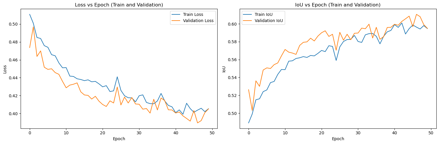
By plotting the Loss functions and mIoU over the training epochs, users can gain insights into potential underfitting or overfitting during training on the train and validation datasets. This comprehensive evaluation helps ensure the robustness and reliability of the model in practical applications.
# Import Libraries
from segmentation_models_pytorch import utils
import torch.optim as optim

best_model = torch.load("./models/best_model.pth", map_location=DEVICE)
metrics = []  # No metrics other than loss for testing

# Define Optimizer (Adam in this case) and learning rate
optimizer = optim.Adam(params=best_model.parameters(), lr=0.0001)

val_epoch = utils.train.ValidEpoch(
    best_model,
    loss=loss,
    metrics=metrics,
    device=DEVICE,
    verbose=True,
)

# Initialize a list to store all test losses
test_losses = []

# Run the validation/testing epoch
for x_test, y_test in tqdm(testDL):
    # Ensure data is on the correct device
    x_test, y_test = x_test.to(DEVICE), y_test.to(DEVICE)

    # Compute loss for the current batch
    test_loss, _ = val_epoch.batch_update(x_test, y_test)

    # Append the current batch's loss to the list of test losses
    test_losses.append(test_loss.item())

# Calculate the average test loss
avg_test_loss = sum(test_losses) / len(test_losses)
The JaccardLoss and IoU over each training epoch can be plotted to assess whether the model is experiencing overfitting or underfitting, and to determine if the learning curve is behaving as expected. In this case, even after 50 epochs, the validation loss closely follows the training loss, indicating that there is no significant overfitting.
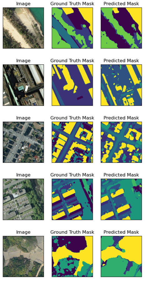
Model Inference
To conclude, the fine-tuned model can then be used for inference to predict segmented masks for the test set. By plotting the original image, the ground truth mask, and the output prediction side-by-side, we can visually assess the model’s performance. As demonstrated below, leveraging transfer learning with a pre-trained model has enabled us to develop a robust segmentation model with commendable accuracy.
Conclusion
This work demonstrates the new functionalities brought by the AI/ML Enhancement Project to guide a ML practitioner through the implementation of transfer learning for EO image segmentation with the following steps:
- Configuring a custom dataset with
pytorchdata loader - Setting up data augmentation to artificially increase the size of a small dataset
- Selecting a pre-trained backbone model for our
Unetmodel - Fine-tune the model
- Model evaluation with
lossfunctions andmIoU - Inference on the unseen
testdataset.
Useful links:
- The link to the Notebook for User Scenario 8 is: https://github.com/ai-extensions/notebooks/blob/main/scenario-8/s8_Transfer_Learning.ipynb
Note: access to this Notebook must be granted - please send an email to support@terradue.com with subject “Request Access to s8_Transfer_Learning.ipynb” and body “Please provide access to Notebook for AI Extensions User Scenario 8” - The user manual of the AI/ML Enhancement Project Platform is available at AI-Extensions Application Hub - User Manual
- Project Update “AI/ML Enhancement Project - Progress Update”
- User Scenario 1 “Exploratory Data Analysis”
- User Scenario 2 “Labelling EO Data”
- User Scenario 3 “Describing labelled EO data”
- User Scenario 4 “Discovering labelled EO data with STAC”
- User Scenario 5 “Developing a new ML model and tracking with MLflow”
- User Scenario 6 “Training and Inference on a remote machine”
- User Scenario 7 “Describing a trained ML model”