AI/ML Enhancement Project - Creating a training dataset
Introduction
In this scenario, the ML practitioner Alice creates a deep learning training dataset. A high-quality, well-annotated dataset is crucial for any AI-driven task; without it, training an effective machine learning (ML) model is doomed to failure. Annotating a dataset is a meticulous and time-consuming process that demands precision and focus. To ensure accuracy, the dataset must be reviewed by multiple experts. However, various computer vision techniques can expedite this process. For instance, an initial labelling can be done by another ML model, with human supervision refining these labels to ensure their correctness.
This post presents User Scenario 9 of the AI/ML Enhancement Project, titled “Alice creates a training dataset”. It demonstrates how the enhancements being deployed in the Geohazards Exploitation Platform (GEP) and Urban Thematic Exploitation Platform (U-TEP) will support users on generating a labelled dataset for a semantic segmentation task in the context of Earth Observation (EO) using both manual and automated ML-driven solutions.
These new capabilities are implemented with an interactive Jupyter Notebook to guide an ML practitioner, such as Alice, through the following steps:
- Import libraries (e.g.,
pystac,rasterio,boto3,sklearn) - Load the Sentinel-2 data using STAC
- Generate Training Dataset using both manual and ML approach
- Create STAC Objects
- Post STAC Objects to a dedicated S3 bucket and then publish on STAC endpoint
Practical examples and commands are displayed to demonstrate how these new capabilities can be used from a Jupyter Notebook or from a dedicated, open-source annotation tool.

Load EO Data with STAC
The EO data used in this scenario were Sentinel-2 data published on the STAC endpoint. More information on this can be found in the related article “Discovering Labelled EO Data with STAC”.
# Import Libraries
import pystac
from pystac_client import Client

catalog = Client.open("https://ai-extensions-stac.terradue.com",
                      headers=get_headers(),ignore_conformance=True)

query = catalog.search(collections=["ai-extensions-svv-dataset-labels"])
eo_items_selected = [item for item in query.item_collection() if any(link.rel == 'source' for link in item.links)]
Generate Training Dataset
The training dataset generated in this Scenario consisted on
- EO data image patches and their corresponding masks
- image patches with their corresponding masks (annotated with three classes
water,non-waterandnot-applicable)
Human-annotation Approach
For demonstrating the process of creating an image segmentation dataset with a manual approach, we used the IRIS Tool. Developed by ESA/ESRIN Phi-Lab, this AI-assisted tool enhances image segmentation and classification for EO imagery and other types of images via a manual human-annotation approach. While this method is more accurate and reliable than automated alternatives, it is also time-consuming and lacks quick reproducibility, making automated methods the preferred choice in those cases. Key highlights of the IRIS Tool are provided below, while a detailed tutorial can be found in IRIS_Tutorial.md.
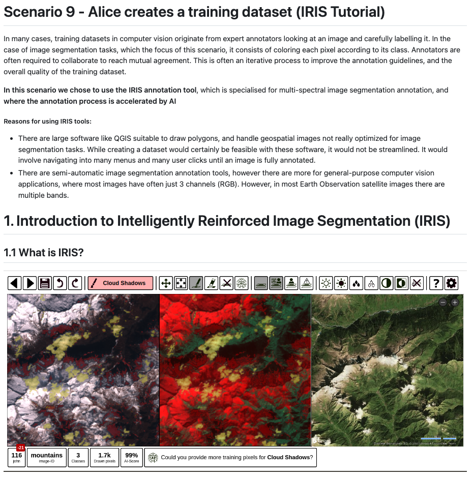
IRIS was designed to streamline the manual creation of ML training datasets for EO by fostering collaboration among multiple annotation experts. It features an iterative process aimed at refining annotation guidelines and enhancing the overall quality of the training dataset. This application is a Flask app that can be deployed both locally and in the cloud, with Github Codespace being the recommended platform for cloud deployment.
As described by the official IRIS project documentation, the highlights of the IRIS tool are:
- Supported by AI model
Gradient Boosted Decision Treefor image segmentation - Multiple and configurable views for multispectral imagery
- Multi-user support: invite multiple annotators to collaborate on the same image segmentation labelling project. This collaborative approach helps merge results and reduces bias and errors, enhancing the accuracy and reliability of the results
- Simple setup with
pipand one configuration file.
The annotation workflow consists of the following steps:
- Annotate just a few pixels: in order to trigger the AI feature to help the annotation process, the user only needs to manually label 10 pixels from 2 classes. This can be done simply by selecting the specific class and then colouring on the pixels that must be assigned to that class on the map, by using the dedicated widgets. An example is shown below, where three classes are labelled with different colours:
WATER(blue),NON-WATER(yellow),NOT-APPLICABLE(red).
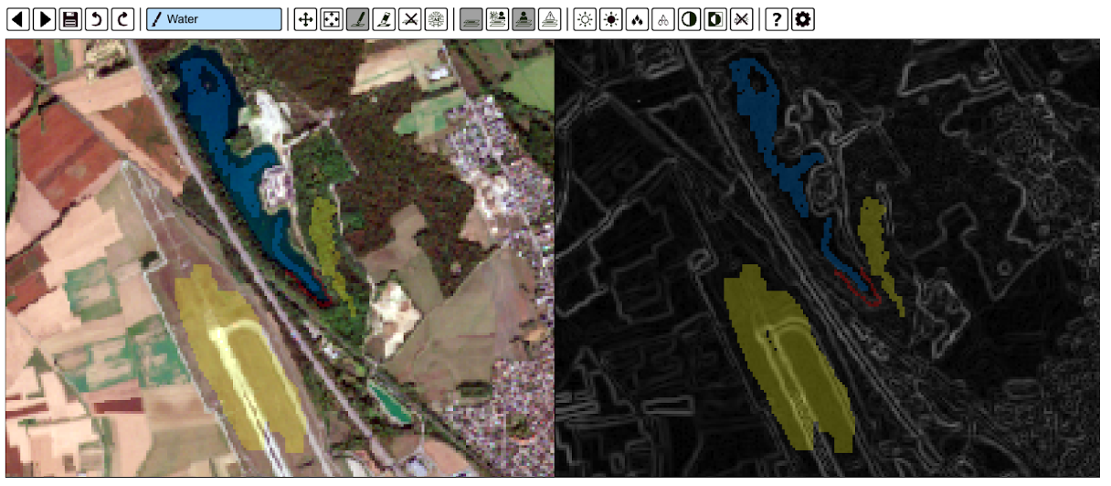
- Train the AI: the
Gradient Boosted Decision Treetraining process can be triggered by the user with the dedicated button. This process is based on the already-annotated pixels in step 1 and is very fast. - Visualise results: based on the annotated pixels, the AI-trained model predictions are shown in the rest of the images. The user can visually inspect the segmentation predictions by moving and zooming in on the image.
- Iterate: If the predicted segmentation needs improvements, the user can proceed by repeating steps 1 to 3 iteratively for manually creating additional labelled pixels. This will increase the quantity of training data for the AI model and will improve the quality of the AI-segmented predictions.
- Save the dataset: When the predicted segmentation results are satisfactory, the user can simply save the predicted image mask, which is saved automatically in the same directory as the input image, in the formats
.png,.npyor.tif, depending on the configuration settings.
Machine Learning Approach
For generating the image segmentation dataset via an automated ML approach we used a model that was previously trained on labelled dataset in Scenario 2 (see related article “Labelling EO Data User Scenario 2”). This consists of a RandomForest model for segmenting a Sentinel-2 image and generating an output water bodies mask with three classes: NON-WATER, WATER, NOT-APPLICABLE. Although this computer vision technique results in masks that are less accurate, the overall accuracy of labels can be improved by manually refining the results using tools such as the IRIS tool. The output dataset resulting from this combined approach can then be leveraged to train a highly accurate segmentation model such as UNET.
The Python library mlflow was used to access the trained models from the MLflow server and to select the best model, based on specific evaluation metrics. The best model was then loaded into this Notebook and then inference on the input EO data was performed to generate the water bodies masks.
# Import Libraries
import mlflow
import json

mlflow.set_tracking_uri(os.environ.get('MLFLOW_TRACKING_URI'))
active_runs = mlflow.search_runs(
    experiment_names = ["water-bodies"],
    # select the best one with highest f1_score and test accuracy
    filter_string="metrics.f1_score > 0.8 AND metrics.test_accuracy>0.98", search_all_experiments=True
).sort_values(by=['metrics.f1_score','metrics.test_accuracy','metrics.precision'],
              ascending=False).reset_index().loc[0]
artifact_path = json.loads(active_runs['tags.mlflow.log-model.history'])[0]['artifact_path']
best_model_path = active_runs.artifact_uri+f'/{artifact_path}'
MODEL = mlflow.pyfunc.load_model(model_uri=best_model_path)
The user defines a DataAcquisition Class that is applied to each input EO data. The Class is responsible for:
- generating image chips from the input EO data
- apply the trained ML model to generate water-bodies masks for each image chip
- create an RGB thumbnail in JPEG format of each image chip.
The data is then stored in the defined output directory. An extraction of the DataAcquisition Class for creating the dataset is shown below.
import tqdm
import rasterio
COMMON_BANDS = ['red','green','blue']
FEATURE_COLUMNS = ['coastal','red','green','blue','nir','nir08',
                   'nir09','swir16','swir22', 'ndvi', 'ndwi1', 'ndwi2']

class DataAcquisition:
    def __init__(self, eo_items: List[pystac.Item], common_bands:List[str], FEATURE_COLUMNS:List[str], model,base_resolution:float=10):
        super().__init__()
        self.eo_items = eo_items
        self.common_bands = common_bands
        self.FEATURE_COLUMNS = FEATURE_COLUMNS
        self.model = model
        self.base_resolution = base_resolution

    def __getitem__(self, idx):
        # Getting source url to sentinel-2 images
        source_sel = self.eo_items[idx].get_links(rel="source")[0].href
        self.band_urls = self.get_image_links(source_sel)

        # Resample bands to the same shape and resolution
        self.band_urls = ml_helper.resample_bands(
            self.band_urls,
            self.base_resolution,
            self.out_dir,
            desired_shape=(10980,10980)
        )

        # Prediction on each image patch to generate the segmented mask
        tif_path = ml_helper.data_and_mask_generator(model = self.model,
                                            band_urls= self.band_urls,
                                            feature_cols=self.FEATURE_COLUMNS,
                                            common_bands= self.common_bands,
                                            out_dir = self.dataset_dir,
                                            eo_item= self.eo_items[idx])

    # Create thumbnail
    def create_thumbnail(self,tif_paths, size=(128, 128)):
        for tiff_path in tqdm(tif_paths,desc="Creating thumbnail"):
            with rasterio.open(tiff_path) as src:
                # Read RGB bands, normalise to 0-255, and save the thumbnail in .jpeg format
                data = src.read()
                data = ((data - data.min()) / (data.max() - data.min()) * 255).astype(np.uint8)
                data = data[:3, :, :]
                data = np.transpose(data, (1, 2, 0))
                image = Image.fromarray(data)
                image.thumbnail(size)
                thumbnail_path = tiff_path.replace(".tif", ".jpeg")
                image.save(thumbnail_path)

# Apply DataAcquisition Class to the input EO data
dataset = DataAcquisition(eo_items=eo_items_selected,common_bands=COMMON_BANDS,
                          FEATURE_COLUMNS=FEATURE_COLUMNS, model= MODEL)
Create STAC Objects
Once all the image masks are created, the user proceeds by creating the STAC Objects (i.e. the STAC Catalog, the STAC Collection and the STAC Items). The assets of each STAC Item describe an image patch, its mask and its thumbnail. More information on the STAC specifications can also be found in the related article “Describing labelled EO Data with STAC”.
# STAC Catalog
catalog_metadata = {
    "id": IMAGES_DIRECTORY,
    "description": "A training dataset for water-bodies segmentation task",
    "catalog_type": pystac.CatalogType.SELF_CONTAINED,
}

# STAC Collection
collection_metadata = {
    "id": IMAGES_DIRECTORY,
    "keywords":["segmentation", "water-bodies","earthsearch"],
    "license": "MIT",
    "provider_name" : "Terradue",
    "provider_role" : ["producer"],  # Any of licensor, producer, processor or host.
    "provider_homepage_url" : "https://www.terradue.com/portal/",

}
# STAC Item
stac_item_properties_common_metadata = {
    "license" : "MIT", # for more license please check https://spdx.org/licenses/
    "provider_name" : "Terradue",
    "provider_role" : "producer",  # Any of licensor, producer, processor or host.
    "provider_homepage_url" : "https://www.terradue.com/portal/",
    "platform" : "ai-extension",
    "instruments" : "MSI",
    "constellation" : "sentinel-2",
    "mission" : "sentinel-2"
}
stac_item_properties_extensions = {
    # Label Extenstion properties
    "class_values": {
        0: "NON-WATER",
        1: "WATER",
        2: "NOT-APPLICABLE"
    },
    "label_tasks" : [LabelTask.SEGMENTATION],
    "label_description": "Water / Non-Water / Not-Applicable",
}
item_metadata = {
    "image_paths": glob(f'{DATASET_PATH}/{IMAGES_DIRECTORY}/**/image_*.tif', recursive=True),
    "mask_paths" : glob(f'{DATASET_PATH}/{IMAGES_DIRECTORY}/**/mask_*.tif', recursive=True),
    "properties":{
    "common_metadata": stac_item_properties_common_metadata,
    "extensions": stac_item_properties_extensions,
}}

# STAC Object generator
stac_generator_obj = stac_helper.StacGenerator(
        DATASET_PATH=DATASET_PATH,
        COMMON_BANDS=COMMON_BANDS,
        IMAGES_DIRECTORY=IMAGES_DIRECTORY,
        item_metadata = item_metadata,
        collection_metadata=collection_metadata,
        catalog_metadata=catalog_metadata)
catalog, collection, stac_items = stac_generator_obj.main()
Post on S3 bucket and publish on STAC endpoint
These two activities - posting the STAC Objects to an S3 bucket and then publishing them on the STAC endpoint - followed the same process described in details in the related articles “Describing labelled EO Data with STAC” and “Describing a trained ML model with STAC”. Please refer to those articles where the steps for each of these activities are explained in great detail.
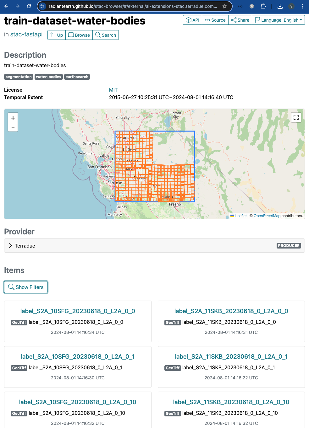
The screenshot below shows the STAC Collection train-dataset-water-bodies published on the endpoint. In addition to the Collection keywords and spatial / temporal extents, a preview of some listed STAC Items is shown underneath the map.
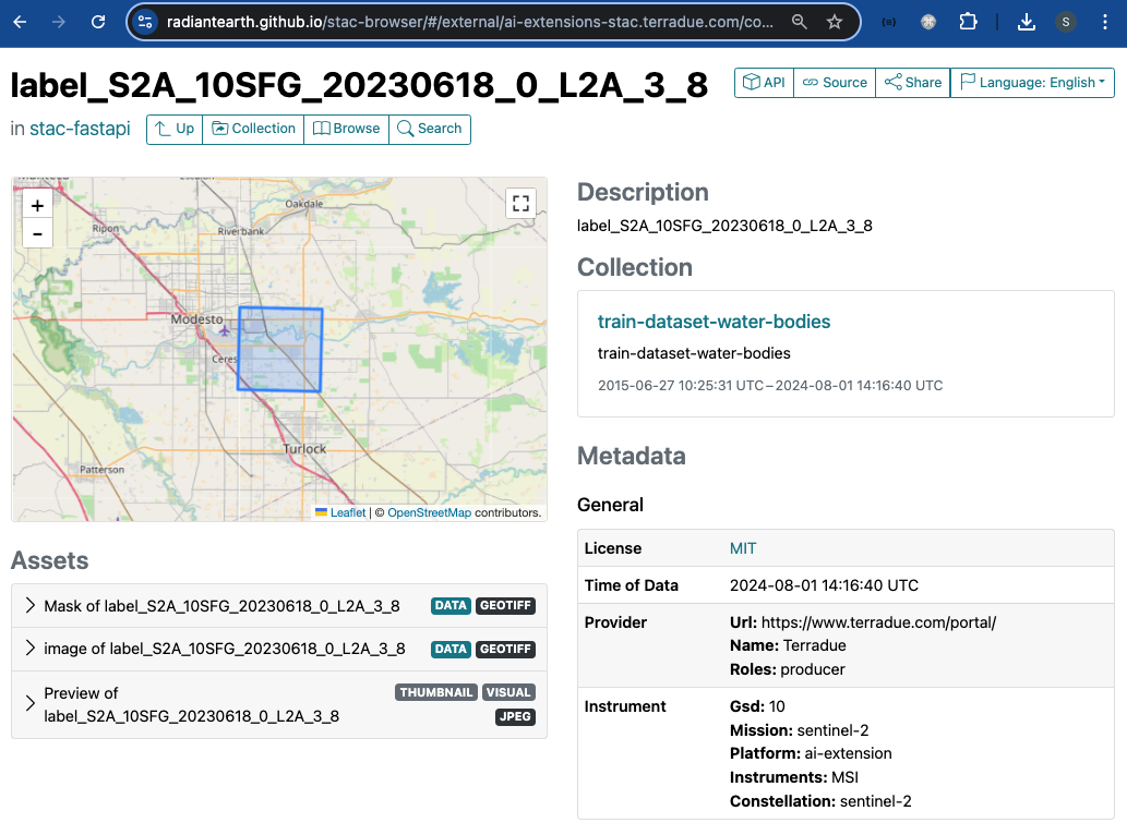
Below is shown a STAC Item as an example. Key features of the STAC Item that are visible in the dashboard are: temporal and spatial extent, description, Collection, key metadata, and the three assets (input image chip, segmented mask, and thumbnail).
Conclusion
This work demonstrates the new functionalities brought by the AI/ML Enhancement Project to guide a ML practitioner through the generation of a labelled EO dataset for a semantic segmentation task using both manual and automated approaches with the following steps:
- Load the Sentinel-2 data using STAC
- Generate Training Dataset using both manual approach (with the IRIS Tool), and automated ML approach
- Create STAC Objects
- Post STAC Objects to a dedicated S3 bucket and then publish on STAC endpoint
Useful links:
- The link to the Notebook for User Scenario 9 is: https://github.com/ai-extensions/notebooks/blob/main/scenario-9/s9-CreatingTrainingData.ipynb
Note: access to this Notebook must be granted - please send an email to support@terradue.com with subject “Request Access to s9-CreatingTrainingData.ipynb” and body “Please provide access to Notebook for AI Extensions User Scenario 9” - The user manual of the AI/ML Enhancement Project Platform is available at AI-Extensions Application Hub - User Manual
- Project Update “AI/ML Enhancement Project - Progress Update”
- User Scenario 1 “Exploratory Data Analysis”
- User Scenario 2 “Labelling EO Data”
- User Scenario 3 “Describing labelled EO data”
- User Scenario 4 “Discovering labelled EO data with STAC”
- User Scenario 5 “Developing a new ML model and tracking with MLflow”
- User Scenario 6 “Training and Inference on a remote machine”
- User Scenario 7 “Describing a trained ML model”
- User Scenario 8 “Reusing an existing pre-trained model”